 SRE文档
SRE文档1. PromQL是什么?
PromQL(Prometheus Query Language)是 Prometheus 自己开发的表达式语言,语言表现力很丰富,内置函数也很多。使用它可以对时序数据进行筛选和聚合。
1.1 组成
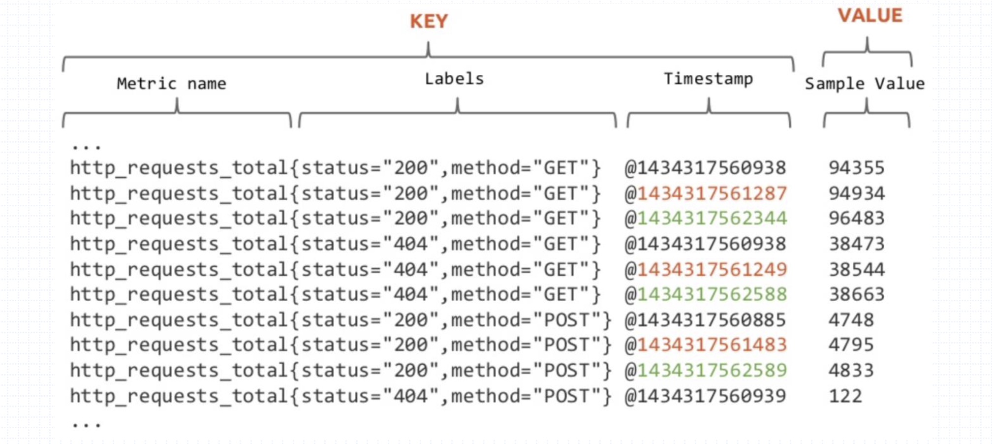
Prometheus会将所有采集到的样本数据以时间序列(time-series)的方式保存在内存数据库中,并且定时保存到硬盘上,每个数据称为一个样本。时间序列(time-series)是按照时间戳和值的序列顺序存放的,我们称之为向量(vector). 每条时间序列(time-series)通过指标名称(metrics name)和一组标签集(labelset)命名。如下所示,可以将时间序列(time-series)理解为将多个时间序列(time-series)放在同一个坐标系内(以时间为横轴,以序列为纵轴),将形成一个由数据点组成的矩阵;
可以把以下图想象成Promethus存储
- 每一行代表一个时间序列(time-series)我们也称为一个向量(Vector)
- 每一列代表时间的流逝时间点
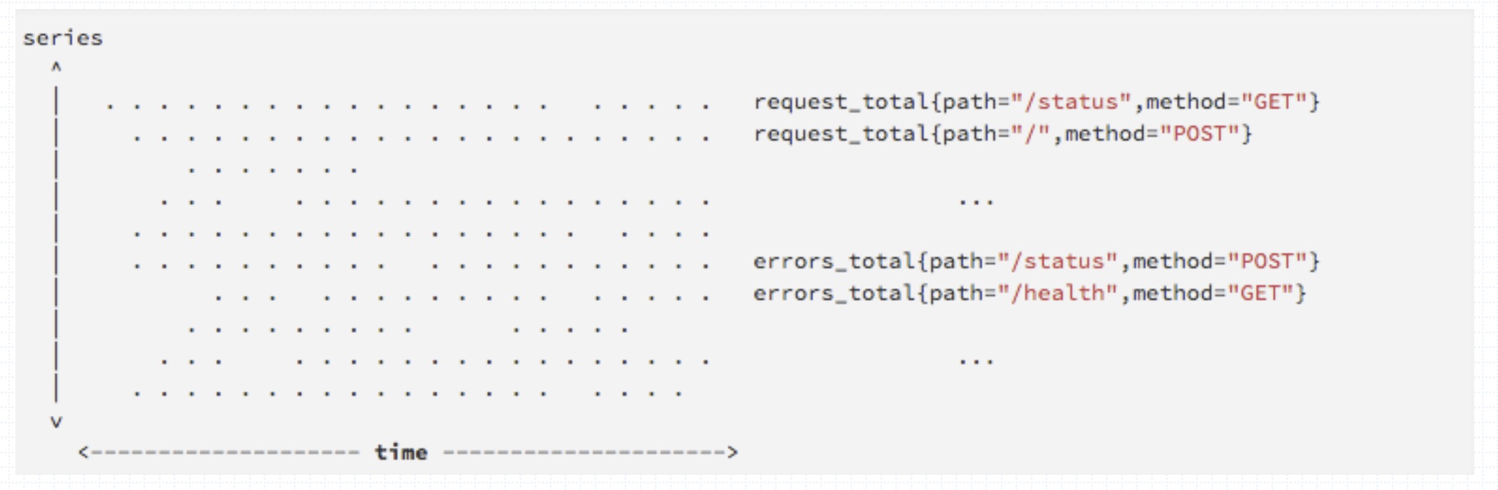
在时间序列(time-series)中的每一个点称为一个样本(sample),样本由以下三部分组成:
- 指标名(metric name):指标名(metric name)和描述当前样本特征的标签(labels);
- 时间戳(timestamp):一个精确到毫秒的时间戳;
- 样本值(value): 一个float64的浮点型数据表示当前样本的值。
1.1 指标类型
包含四种指标类型
- counter(计数器)
- gauge (仪表类型)
- histogram(直方图类型)
- summary (摘要类型)
1.counter(计数器)
Counter (只增不减的计数器) 类型的指标其工作方式和计数器一样,只增不减。常见的监控指标,如 http_requests_total、 node_cpu_seconds_total 都是 Counter 类型的监控指标。
比如:
# HELP node_cpu_seconds_total Seconds the cpus spent in each mode.
# TYPE node_cpu_seconds_total counter
node_cpu_seconds_total{cpu="cpu0",mode="idle"} 362812.7890625
# HELP node_cpu_seconds_total Seconds the cpus spent in each mode.
# TYPE node_cpu_seconds_total counter
node_cpu_seconds_total{cpu="cpu0",mode="idle"} 362812.7890625#HELP:解释当前指标的含义,上面表示在每种模式下 node 节点的 cpu 花费的时间,以 s 为单位。#TYPE:说明当前指标的数据类型,上面是 counter 类型。
2.gauge (仪表类型)
与 Counter 不同, Gauge(可增可减的仪表盘)类型的指标侧重于反应系统的当前状态。因此这类指标的样本数据可增可减。常见指标如:node_memory_MemFree_bytes(主机当前空闲的内存大小)、 node_memory_MemAvailable_bytes(可用内存大小)都是 Gauge 类型的监控指标。通过 Gauge 指标,用户可以直接查看系统的当前状态:
node_memory_MemFree_bytesnode_memory_MemFree_bytes对于 Gauge 类型的监控指标,通过 PromQL 内置函数,使用 predict_linear() 对数据的变化趋势进行预测。例如,预测系统磁盘空间在 4 个小时之后的剩余情况:
predict_linear(node_filesystem_free_bytes[1h], 4 * 3600)predict_linear(node_filesystem_free_bytes[1h], 4 * 3600)4.Histogram(直方图类型) 和 Summary(摘要类型)
Histogram 和 Summary 主用用于统计和分析样本的分布情况
指标 prometheus_tsdb_wal_fsync_duration_seconds 的指标类型为 Summary。它记录了 Prometheus Server 中 wal_fsync 的处理时间,通过访问 Prometheus Server 的 /metrics 地址,可以获取到以下监控样本数据:
# HELP prometheus_tsdb_wal_fsync_duration_seconds Duration of WAL fsync.
# TYPE prometheus_tsdb_wal_fsync_duration_seconds summary
prometheus_tsdb_wal_fsync_duration_seconds{quantile="0.5"} 0.012352463
prometheus_tsdb_wal_fsync_duration_seconds{quantile="0.9"} 0.014458005
prometheus_tsdb_wal_fsync_duration_seconds{quantile="0.99"} 0.017316173
prometheus_tsdb_wal_fsync_duration_seconds_sum 2.888716127000002
prometheus_tsdb_wal_fsync_duration_seconds_count 216
# HELP prometheus_tsdb_wal_fsync_duration_seconds Duration of WAL fsync.
# TYPE prometheus_tsdb_wal_fsync_duration_seconds summary
prometheus_tsdb_wal_fsync_duration_seconds{quantile="0.5"} 0.012352463
prometheus_tsdb_wal_fsync_duration_seconds{quantile="0.9"} 0.014458005
prometheus_tsdb_wal_fsync_duration_seconds{quantile="0.99"} 0.017316173
prometheus_tsdb_wal_fsync_duration_seconds_sum 2.888716127000002
prometheus_tsdb_wal_fsync_duration_seconds_count 216类型为 Histogram 的监控指标 prometheus_tsdb_compaction_chunk_range_seconds_bucket
# HELP prometheus_tsdb_compaction_chunk_range_seconds Final time range of chunks on their first compaction
# TYPE prometheus_tsdb_compaction_chunk_range_seconds histogram
prometheus_tsdb_compaction_chunk_range_seconds_bucket{le="100"} 71
prometheus_tsdb_compaction_chunk_range_seconds_bucket{le="400"} 71
prometheus_tsdb_compaction_chunk_range_seconds_bucket{le="1600"} 71
prometheus_tsdb_compaction_chunk_range_seconds_bucket{le="6400"} 71
prometheus_tsdb_compaction_chunk_range_seconds_bucket{le="25600"} 405
prometheus_tsdb_compaction_chunk_range_seconds_bucket{le="102400"} 25690
prometheus_tsdb_compaction_chunk_range_seconds_bucket{le="409600"} 71863
prometheus_tsdb_compaction_chunk_range_seconds_bucket{le="1.6384e+06"} 115928
prometheus_tsdb_compaction_chunk_range_seconds_bucket{le="6.5536e+06"} 2.5687892e+07
prometheus_tsdb_compaction_chunk_range_seconds_bucket{le="2.62144e+07"} 2.5687896e+07
prometheus_tsdb_compaction_chunk_range_seconds_bucket{le="+Inf"} 2.5687896e+07
prometheus_tsdb_compaction_chunk_range_seconds_sum 4.7728699529576e+13
prometheus_tsdb_compaction_chunk_range_seconds_count 2.5687896e+07
# HELP prometheus_tsdb_compaction_chunk_range_seconds Final time range of chunks on their first compaction
# TYPE prometheus_tsdb_compaction_chunk_range_seconds histogram
prometheus_tsdb_compaction_chunk_range_seconds_bucket{le="100"} 71
prometheus_tsdb_compaction_chunk_range_seconds_bucket{le="400"} 71
prometheus_tsdb_compaction_chunk_range_seconds_bucket{le="1600"} 71
prometheus_tsdb_compaction_chunk_range_seconds_bucket{le="6400"} 71
prometheus_tsdb_compaction_chunk_range_seconds_bucket{le="25600"} 405
prometheus_tsdb_compaction_chunk_range_seconds_bucket{le="102400"} 25690
prometheus_tsdb_compaction_chunk_range_seconds_bucket{le="409600"} 71863
prometheus_tsdb_compaction_chunk_range_seconds_bucket{le="1.6384e+06"} 115928
prometheus_tsdb_compaction_chunk_range_seconds_bucket{le="6.5536e+06"} 2.5687892e+07
prometheus_tsdb_compaction_chunk_range_seconds_bucket{le="2.62144e+07"} 2.5687896e+07
prometheus_tsdb_compaction_chunk_range_seconds_bucket{le="+Inf"} 2.5687896e+07
prometheus_tsdb_compaction_chunk_range_seconds_sum 4.7728699529576e+13
prometheus_tsdb_compaction_chunk_range_seconds_count 2.5687896e+07与 Summary 类型的指标相似之处在于 Histogram 类型的样本同样会反应当前指标的记录的总数(以 _count 作为后缀)以及其值的总量(以 _sum 作为后缀)。不同在于 Histogram 指标直接反应了在不同区间内样本的个数,区间通过标签 le 进行定义。
2. PromQL语法
2.1 数据类型
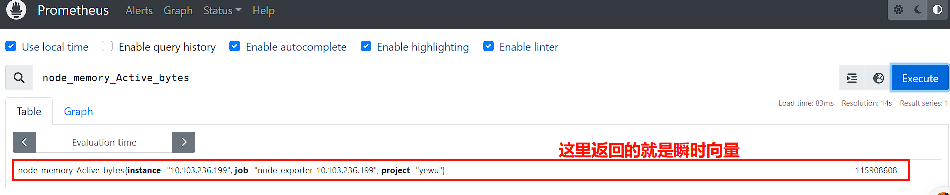
1.瞬时向量-Instant vector
瞬时向量 (Instant vector): 一组时序,每个时序只有一个采样值
比如:node_memory_Active_bytes
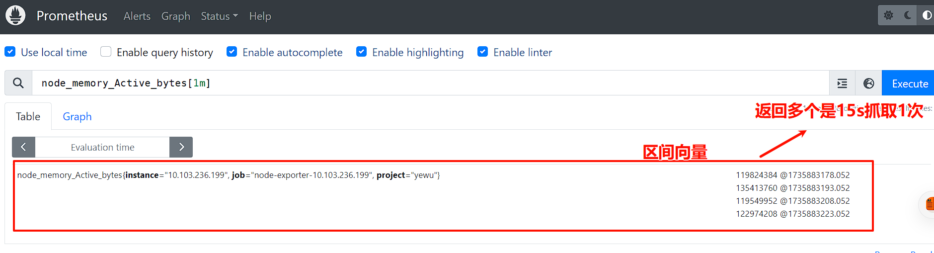
2.区间向量-Range vector
区间向量 (Range vector): 一组时序,每个时序包含一段时间内的多个采样值
比如:node_memory_Active_bytes[1m]
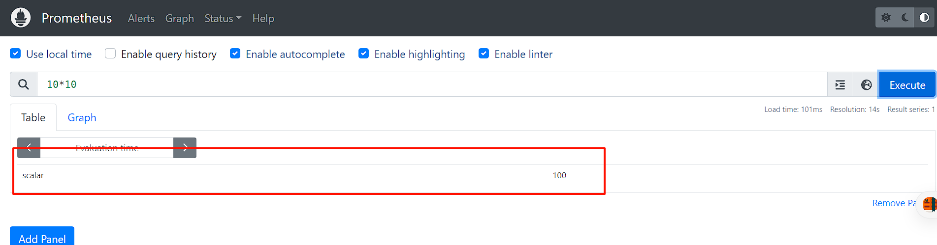
3.标量数据-Scalar
标量数据 (Scalar): 一个浮点数
比如:10*10
❌ 注意
需要注意的是,当使用表达式count(http_requests_total),返回的数据类型,依然是瞬时向量。用户可以通过内置函数scalar将单个瞬时向量转换为标量。
4.字符串-String
字符串 (String): 一个字符串,暂时未用
字符串可以用单引号,双引号或反引号指定为文字,如果字符串内的特殊符号想要生效,我们可以使用反引号。
"this is a string"
'these are unescaped: n t'
`these are not unescaped: n ' " t`
字符串可以用单引号,双引号或反引号指定为文字,如果字符串内的特殊符号想要生效,我们可以使用反引号。
"this is a string"
'these are unescaped: n t'
`these are not unescaped: n ' " t`2.2 时序选择器
1.瞬时向量选择器
瞬时向量选择器用来选择一组时序在某个采样点的采样值
比如:拿node_cpu_seconds_total举例
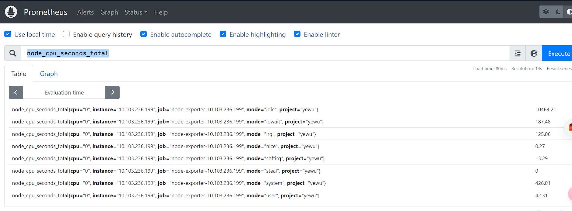
可以通过在后面添加用大括号包围起来的一组标签键值对来对时序进行过滤。
比如表达式,node_cpu_seconds_total
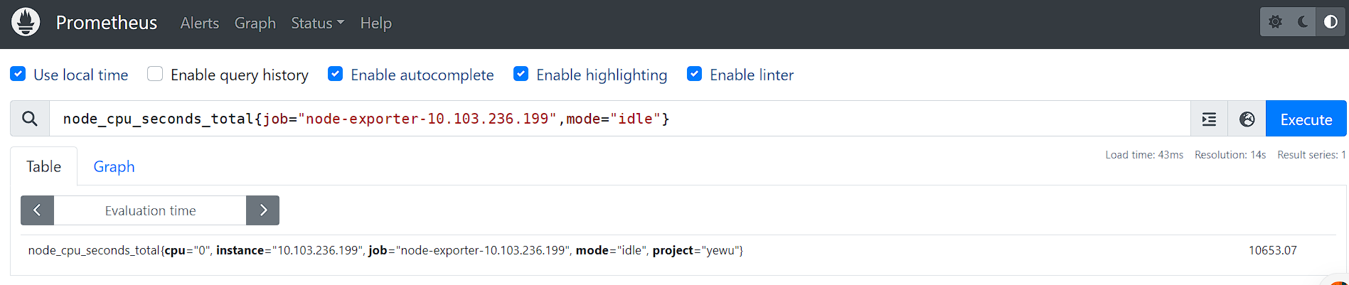
匹配标签值时可以是等于,也可以使用正则表达式。总共有下面几种匹配操作符:
=:完全相等!=: 不相等=~: 正则表达式匹配!~: 正则表达式不匹配
度量指标名可以使用内部标签 __name__ 来匹配,表达式 node_cpu_seconds_total 也可以写成 {__name__="node_cpu_seconds_total"}。表达式 {__name__=~"job:.*"} 匹配所有度量指标名称以 job: 打头的时序。
2.区间向量选择器
区间向量选择器类似于瞬时向量选择器,不同的是它选择的是过去一段时间的采样值。可以通过在瞬时向量选择器后面添加包含在 [] 里的时长来得到区间向量选择器。比如下面的表达式选出了所有度量指标为 node_cpu_seconds_total 且 job 为 prometheus 的时序在过去 5 分钟的采样值。
比如:
node_cpu_seconds_total{job="node-exporter-10.103.236.199"}[1m]node_cpu_seconds_total{job="node-exporter-10.103.236.199"}[1m]说明:时长的单位可以是下面几种之一:
- s:seconds
- m:minutes
- h:hours
- d:days
- w:weeks
- y:years
❌ 注意
注意: 范围向量选择器返回的是一定时间范围内的数据样本,虽然不同时间序列的数据抓取时间点相同,但它们的时间戳并不会严格对齐;
多个Target上的数据抓取需要分散在抓取时间点前后一定的时间范围内,以均衡Prometheus Server的负载;
因而,Prometheus在趋势上准确,但并非绝对精准;
3.偏移修饰器
前面介绍的选择器默认都是以当前时间为基准时间,偏移修饰器用来调整基准时间,使其往前偏移一段时间。偏移修饰器紧跟在选择器后面,使用 offset 来指定要偏移的量。比如下面的表达式选择度量名称为 node_cpu_seconds_total 的所有时序在 5 分钟前的采样值。
比如:
node_cpu_seconds_total offset 1mnode_cpu_seconds_total offset 1m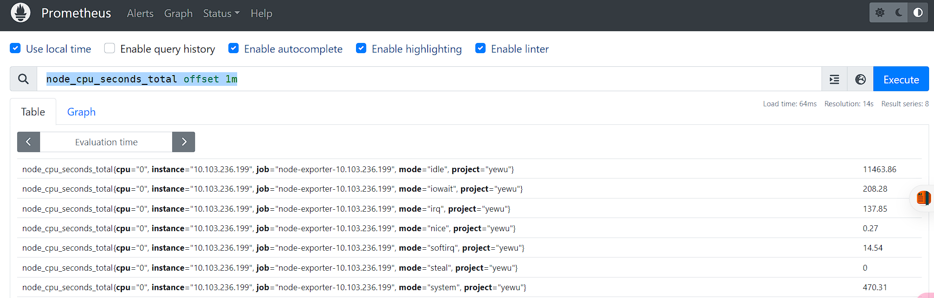
还比如,下面的表达式选择 node_cpu_seconds_total 度量指标在 1 周前的这个时间点过去 5 分钟的采样值
node_cpu_seconds_total[5m] offset 1wnode_cpu_seconds_total[5m] offset 1w❌ 注意
注意: offset 与 数据选择器是一个整体,不能分割 offset 偏移的是时间点